Contents
Learning Sources
Books
http://www.feat.engineering/
Readings & Videos
machine learning

https://youtu.be/jGwO_UgTS7I?list=PLoROMvodv4rMiGQp3WXShtMGgzqpfVfbU

https://www.youtube.com/@NeoWizard
scklearn

https://www.youtube.com/watch?v=eVxGhCRN-xA&pp=ygUQ7YyM7J207I2sIOqwleydmA%3D%3D
https://youtu.be/eVxGhCRN-xA
https://youtu.be/pqNCD_5r0IU
https://www.youtube.com/watch?v=URTZ2jKCgBc&list=PLQVvvaa0QuDd0flgGphKCej-9jp-QdzZ3
https://www.youtube.com/@NeoWizard
https://youtu.be/TNcfJHajqJY
ML 101
Feature engineerings
feature engineering – the process of creating representations of data that increase the effectiveness of a model. ( from “Feature Engineering and Selection: A Practical Approach for Predictive Models” Max Kuhn and Kjell Johnson, 2019)
When two features are highly correlated, problems may arise in some models (e.g., simple regressions,
Ttrack outliers in the summary statistics (when the maximum/median or median/minimum ratios seem suspicious).
In the machine learning algorithm, explain the concept of conditional average in feature engineering.
In machine learning, the concept of “conditional average” in feature engineering refers to computing the average value of a target variable or another feature, conditioned on the values of one or more specific features. This technique can be used to create new features that capture the relationship between these features and the target variable.
Steps to Calculate Conditional Average
- Identify the Variables:
- Target Variable (Y): The variable for which the conditional average will be computed.
- Conditioning Features (X): The features on which the conditional average of Y will be conditioned.
- Group Data by Conditioning Features:
- Partition the dataset based on unique values or ranges of the conditioning features.
- Compute the Average:
- For each group formed in the previous step, compute the average value of the target variable (or the feature of interest).
- Assign the Conditional Average:
- Create a new feature in the dataset where each instance is assigned the conditional average computed for its group.
Example
Suppose you have a dataset with the following features:
- Feature X1: Age of a customer
- Feature X2: Gender of a customer
- Target Variable Y: Annual spending amount
You want to create a new feature that captures the average annual spending conditioned on the age and gender of the customers.
Step-by-Step Calculation
- Identify the Variables:
- Target Variable (Y): Annual spending amount.
- Conditioning Features (X): Age and Gender.
- Group Data by Conditioning Features:
- Partition the dataset by unique combinations of Age and Gender.
- Compute the Average:
- For each age-gender combination, compute the average annual spending amount.
- Assign the Conditional Average:
- Create a new feature, say “Cond_Avg_Spending,” and for each customer, assign the computed average spending amount based on their age and gender group.
Example Dataset
| Age | Gender | Annual Spending | Cond_Avg_Spending |
|---|---|---|---|
| 25 | Male | $2000 | $2200 |
| 30 | Female | $3000 | $2800 |
| 25 | Male | $2400 | $2200 |
| 30 | Female | $2600 | $2800 |
Here, “Cond_Avg_Spending” is the conditional average of annual spending based on the customer’s age and gender.
Applications
- Handling Categorical Variables: Creating conditional averages for categorical variables to capture their impact on the target variable.
- Reducing Noise: Smoothing noisy features by computing averages over groups.
- Capturing Relationships: Enhancing model performance by capturing complex relationships between features and the target variable.
Implementation in Python (Pandas Example)
import pandas as pd# Sample data
data = {

'Age': [25, 30, 25, 30],

'Gender': ['Male', 'Female', 'Male', 'Female'],
'Annual_Spending': [2000, 3000, 2400, 2600]
}
df = pd.DataFrame(data)
# Compute conditional average
df['Cond_Avg_Spending'] = df.groupby(['Age', 'Gender'])['Annual_Spending'].transform('mean')
print(df)
This will output:
Age Gender Annual_Spending Cond_Avg_Spending
25 Male 2000.0 2200.0 30 Female 3000.0 2800.0 25 Male 2400.0 2200.0 30 Female 2600.0 2800.0
The new feature “Cond_Avg_Spending” captures the conditional average annual spending based on the age and gender of the customers.
Sklearn modules
| 모듈 | 설명 |
|---|---|
sklearn.datasets |
내장된 예제 데이터 세트 |
sklearn.preprocessing |
다양한 데이터 전처리 기능 제공 (변환, 정규화, 스케일링 등) |
sklearn.feature_selection |
특징(feature)를 선택할 수 있는 기능 제공 |
sklearn.feature_extraction |
특징(feature) 추출에 사용 |
sklearn.decomposition |
차원 축소 관련 알고리즘 지원 (PCA, NMF, Truncated SVD 등) |
sklearn.model_selection |
교차 검증을 위해 데이터를 학습/테스트용으로 분리, 최적 파라미터를 추출하는 API 제공 (GridSearch 등) |
sklearn.metrics |
분류, 회귀, 클러스터링, Pairwise에 대한 다양한 성능 측정 방법 제공 (Accuracy, Precision, Recall, ROC-AUC, RMSE 등) |
sklearn.pipeline |
특징 처리 등의 변환과 ML 알고리즘 학습, 예측 등을 묶어서 실행할 수 있는 유틸리티 제공 |
sklearn.linear_model |
선형 회귀, 릿지(Ridge), 라쏘(Lasso), 로지스틱 회귀 등 회귀 관련 알고리즘과 SGD(Stochastic Gradient Descent) 알고리즘 제공 |
sklearn.svm |
서포트 벡터 머신 알고리즘 제공 |
sklearn.neighbors |
최근접 이웃 알고리즘 제공 (k-NN 등) |
sklearn.naive_bayes |
나이브 베이즈 알고리즘 제공 (가우시안 NB, 다항 분포 NB 등) |
sklearn.tree |
의사 결정 트리 알고리즘 제공 |
sklearn.ensemble |
앙상블 알고리즘 제공 (Random Forest, AdaBoost, GradientBoost 등) |
sklearn.cluster |
비지도 클러스터링 알고리즘 제공 (k-Means, 계층형 클러스터링, DBSCAN 등) |
https://www.youtube.com/watch?v=SmZmBKc7Lrs
#Loading the data
from sklearn import datasets
X, y = datasets.load_wine(return_X_y=True)       # Classification

from sklearn import datasets
diabetes = datasets.load_diabetes()              # Regression
X, y = diabetes.data, diabetes.target
# Split to training and testing
from sklearn.model_selection import train_test_split
X_train, X_test, y_train, y_test = train_test_split(X, y, test_size=0.4, random_state=0)
#Preprocessing

Standardization
from sklearn.preprocessing import StandardScaler
scaler = StandardScaler()
scaled_X_train = scaler.fit_transform(X_train)
scaled_X_test = scaler.transform(X_test)

Normalization
from sklearn.preprocessing import Normalizer
norm = Normalizer()
norm_X_train = norm.fit_transform(X_train)
norm_X_test = norm.transform(X_test)

Binarization
from sklearn.preprocessing import Binarizer
binary = Binarizer(threshold=0.0)
binary_X = binary.fit_transform(X)

Encoding Categorical Features
Encode categorical features with string value
from sklearn.preprocessing import LabelEncoder
lab_enc = LabelEncoder()
y = lab_enc.fit_transform(y)

Imputer
from sklearn.impute import SimpleImputer
imp_mean = SimpleImputer(missing_values=0, strategy='mean')
imp_mean.fit_transform(X_train)

Generating Polynomial Features
from sklearn.preprocessing import PolynomialFeatures
poly = PolynomialFeatures(5)
poly.fit_transform(X)
# FIT THE SUPERVISED LEARNING MODEL
from sklearn.linear_model import LinearRegression
from sklearn.linear_model import LogisticRegression
from sklearn.naive_bayes import GaussianNB
from sklearn.neighbors import KNeighborsClassifier
from sklearn.ensemble import RandomForestClassifier
from sklearn.ensemble import GradientBoostingClassifier
from sklearn.svm import SVC

lr = LinearRegression()
lr.fit(X_train, y_train)

knn.fit(X_train, y_train)

svm_svc = SVC(kernel='linear')
svm_svc.fit(X_train, y_train)

gnb = GaussianNB()


# PREDICT Supervised Estimators
y_pred = lr.predict(X_test)
y_pred = svm_svc.predict(X_test)
y_pred = knn.predict_proba(X_test)             #Estimate probability of a label
# FIT THE UNSUPERVISED LEARNING MODEL
from sklearn.decomposition import PCA
from sklearn.cluster import DBSCAN
from sklearn.cluster import AgglomerativeClustering
from sklearn.cluster import KMeans

kmeans = KMeans(n_clusters=5, random_state=0)
kemans_model = k_means.fit(X_train) #Fit the model to the data
pca = PCA(n_components=2)
pca_model = pca.fit_transform(X_train)      #Fit to data, then transform it

# PREDICT Unsupervised Estimators
y_pred = kmeans_model.predict(X_test)       #Predict labels in clustering algos
# FIT THE NN LEARNING MODEL
from sklearn.neural_network import MLPClassifier
from sklearn.neural_network import MLPRegressor
# EVAULATION
from sklearn import metrics

Classfication
Accuracy score
lr.score(X_test, y_test)
from sklearn.metrics import accuracy_score
accuracy_score(y_test, y_pred)

Accuracy Score
>>> knn.score(X_test, y_test)                      #Estimator score method
>>> from sklearn.metrics import accuracy_score     #Metric scoring functions Classification Report
>>> accuracy_score(y_test, y_pred)

Classification Report
>>> from sklearn.metrics import classification_report
>>> print(classification_report(y_test, y_pred))   #Precision, recall, f1-scoreand support

Confusion Matrix
>>> from sklearn.metrics import confusion_matrix
>>> print(confusion_matrix(y_test, y_pred))

Regression Metrics
Mean Squared Error
from sklearn.metrics import mean_squared_error
mean_squared_error(y_test, y_pred)

Mean Absolute Error
>>> from sklearn.metrics import mean_absolute_error
>>> y_true = [3, -0.5, 2]
>>> mean_absolute_error(y_true, y_pred)

R2
Score from sklearn.metrics import r2_score
r2_score(y_test, y_pred)

Clustering Metrics
Adjusted Rand Index
>>> from sklearn.metrics import adjusted_rand_score
>>> adjusted_rand_score(y_true, y_pred)

Homogeneity
>>> from sklearn.metrics import homogeneity_score
>>> homogeneity_score(y_true, y_pred)

V-measure
>>> from sklearn.metrics import v_measure_score
>>> metrics.v_measure_score(y_true, y_pred)
# Cross-validation
from sklearn.model_selection import cross_val_score
cross_val_score(lr, X, y, cv=5, scoring='f1_macro')

from sklearn.cross_validation import cross_val_score
print(cross_val_score(knn, X_train, y_train, cv=4))
print(cross_val_score(lr, X, y, cv=2))
# Model tuning
Grid Search
from sklearn.model_selection import GridSearchCV
parameters = {'kernel':('linear', 'rbf'), 'C':[1, 10]}
model = GridSearchCV(svm_svc, parameters)
model.fit(X_train, y_train)
print(model.best_score_)
print(model.best_estimator_)

>>> from sklearn.grid_search import GridSearchCV
>>> params = { : np.arange(1,3), : [ , ]}
>>> grid = GridSearchCV(estimator=knn, param_grid=params)
>>> grid.fit(X_train, y_train) >>> print(grid.best_score_)
>>> print(grid.best_estimator_.n_neighbors)

Randomized Parameter Optimization
>>> from sklearn.grid_search import RandomizedSearchCV
>>> params = { : range(1,5), : [ , ]}
>>> rsearch = RandomizedSearchCV(estimator=knn, param_distributions=params, cv=4, n_iter=8,random_state=5)
>>> rsearch.fit(X_train, y_train) >>> print(rsearch.best_score_)
# Perform variance thresholding on raw features
from sklearn.feature_selection import VarianceThreshold
# replace each attribute’s missing values with the median of that
attribute:

from sklearn.impute import SimpleImputer
imputer = SimpleImputer(strategy="median")
# convert these categories from text to numbers
from sklearn.preprocessing import OrdinalEncoder
data_encoded = OrdinalEncoder().fit_transform(data)

# OneHotEncoder class to convert categorical values into one-hot vectors
from sklearn.preprocessing import OneHotEncoder
data_encoded = OneHotEncoder().fit_transform(data)
Regression
# linear regression

# training
from sklearn import linear_model
regr = linear_model.LinearRegression()
regr.fit(train_x, train_y)

print ('Intercept: ', regr.intercept_)
print ('Coefficients: ', regr.coef_)

# prediction
test_y_ = regr.predict(test_x)

# evaluatioin
from sklearn.metrics import r2_score

print("Mean absolute error: %.2f" % np.mean(np.absolute(test_y_ - test_y)))
print("Residual sum of squares (MSE): %.2f" % np.mean((test_y_ - test_y) ** 2))
print("R2-score: %.2f" % r2_score(test_y , test_y_) )
# Polynomial regression
from sklearn.preprocessing import PolynomialFeatures
poly_features = PolynomialFeatures(degree=2, include_bias=False)
X_poly = poly_features.fit_transform(X)

lin_reg = LinearRegression()
lin_reg.fit(X_poly, y)
lin_reg.intercept_, lin_reg.coef_
# stochastic gradient dscent

from sklearn.linear_model import SGDRegressor
sgd_reg = SGDRegressor(max_iter=1000, tol=1e-3, penalty=None, eta0=0.1)
sgd_reg.fit(X, y.ravel())
# Ridge
from sklearn.linear_model import Ridge
ridge_reg = Ridge(alpha=1, solver="cholesky")
ridge_reg.fit(X, y)
ridge_reg.predict([[1.5]]


# Lasso
from sklearn.linear_model import Lasso
lasso_reg = Lasso(alpha=0.1)
lasso_reg.fit(X, y)
lasso_reg.predict([[1.5]]
# Elastic net
from sklearn.linear_model import ElasticNet
elastic_net = ElasticNet(alpha=0.1, l1_ratio=0.5)
elastic_net.fit(X, y)
elastic_net.predict([[1.5]])
# Logistic regresion
from sklearn.linear_model import LogisticRegression
logi_reg = LogisticRegression()
logi_reg.fit(X, y)
logi_reg.predict([[1.7], [1.5]])

# logistic with GridSearch
from sklearn.linear_model import LogisticRegression
from sklearn.model_selection import GridSearchCV
lr = LogisticRegression()
parameters = {'C': [0.001, 0.01, 0.1, 1, 10, 100, 1000]}
cv = GridSearchCV(lr, parameters, cv=5)
cv.fit(features, labels)
# Softmax regression
softmax_reg = LogisticRegression(multi_class="multinomial",solver="lbfgs", C=10)
softmax_reg.fit(X, y)
softmax_reg.predict([[5, 2]])
softmax_reg.predict_proba([[5, 2]])
Penalized Regression
resort to penalizations to improve the robustness of factor-based predictive regressions. The outcome can then be used to fuel an allocation scheme. For instance, Han et al. (2019) and Rapach and Zhou (2019) use penalized regressions to improve stock return prediction when combining forecasts that emanate from individual characteristics.
Similar ideas can be developed for macroeconomic predictions for instance, as in Uematsu and Tanaka (2019). The second application stems from a less known result which originates from Stevens (1998). It links the weights of optimal mean-variance portfolios to particular cross-sectional regressions. The idea is then different and the purpose is to improve the quality of mean-variance driven portfolio weights. We present the two approaches below after an introduction on regularization techniques for linear models.
Other examples of financial applications of penalization can be found in d’Aspremont (2011), Ban, El Karoui, and Lim (2016) and Kremer et al. (2019). In any case, the idea is the same as in the seminal paper Tibshirani (1996): standard (unconstrained) optimization programs may lead to noisy estimates, thus adding a structuring constraint helps remove some noise (at the cost of a possible bias). For instance, Kremer et al. (2019) use this concept to build more robust mean-variance (Markowitz (1952)) portfolios and Freyberger, Neuhierl, and Weber (2020) use it to single out the characteristics that help explain the cross-section of equity returns.
Source: “Machine Learning for Factor Investing” by Coqueret and Guida, 2023, CH 5, Chapman & Hall
Tibshirani (1996) is the inventor of LASSO: https://webdoc.agsci.colostate.edu/koontz/arec-econ535/papers/Tibshirani%20(JRSS-B%201996).pdf
“The ‘lasso’ minimizes residual sum of squares subject to the sum of the absolute value of the coefficients being less than a constant”
$latex \underset{\beta_0, \beta}{\text{minimize}} \left( \frac{1}{2N} \sum_{i=1}^{N} \left( y_i – \beta_0 – \sum_{j=1}^{p} \beta_j x_{ij} \right)^2 + \lambda \sum_{j=1}^{p} |\beta_j| \right)$
Lambda is the penalty term that denotes the amount of shrinkage (or constraint) that will be implemented in the equation. With Lambda set to zero, you will find that this is the equivalent of the linear regression model, and a larger value penalizes the optimization function. Therefore, lasso regression shrinks the coefficients and helps to reduce the model complexity and multi-collinearity. Lambda can be any real-valued number between zero and infinity; the larger the value, the more aggressive the penalization is.
A hyperparameter is used called “lambda” that controls the weighting of the penalty to the loss function. A default value of 1.0 will give full weightings to the penalty; a value of 0 excludes the penalty. Very small values of lambda, such as 1e-3 or smaller, are common.
This has the effect of shrinking the coefficients for those input variables that do not contribute much to the prediction task. This penalty allows some coefficient values to go to the value of zero, allowing input variables to be effectively removed from the model, providing a type of automatic feature selection. One approach to address the stability of regression models is to change the loss function to include additional costs for a model that has large coefficients. Linear regression models that use these modified loss functions during training are referred to collectively as penalized linear regression.
https://en.wikipedia.org/wiki/Lasso_(statistics)
https://www.datacamp.com/tutorial/tutorial-lasso-ridge-regression
penalizing the magnitude of coefficients of features and minimizing the error between predicted and actual observations. These are called ‘regularization’ techniques.
LASSO is a type of linear regression that uses shrinkage. Shrinkage is where data values are shrunk towards a central point, like the mean. The LASSO technique uses L1 regularization to penalize the absolute size of the coefficients. This has the effect of setting some coefficients to zero, effectively selecting a simpler model that retains only the most significant features.
Key Points:
- Regularization: LASSO adds a penalty equal to the absolute value of the magnitude of coefficients.
- Feature Selection: By shrinking some coefficients to zero, LASSO can select a subset of features, which is useful for models with many predictors.
- Bias-Variance Tradeoff: Regularization reduces variance but increases bias, which can lead to better model generalization.
LASSO (Least Absolute Shrinkage and Selection Operator) and OLS (Ordinary Least Squares) are both linear regression methods, but they differ significantly in how they handle model complexity and feature selection.
Objective: OLS aims to minimize the sum of squared residuals (the difference between observed and predicted values).
Penalty: OLS does not apply any penalty to the coefficients. As a result, it can lead to overfitting, especially when dealing with many predictors or highly correlated predictors.
Feature Selection: OLS does not perform feature selection. All predictors are included in the final model, regardless of their significance.
Objective: LASSO aims to minimize the sum of squared residuals with an added penalty proportional to the sum of the absolute values of the coefficients.
Penalty: LASSO applies an L1 penalty, which shrinks some coefficients to zero. This can help prevent overfitting and improve the model’s ability to generalize to new data.
Feature Selection: LASSO performs feature selection by setting some coefficients exactly to zero. This means that it effectively selects a simpler model that includes only the most relevant predictors.
By introducing regularization, LASSO balances the complexity of the model and improves its performance on unseen data, addressing the overfitting issue inherent in OLS.
# from Chat GPT
import numpy as np
import pandas as pd
from sklearn.model_selection import train_test_split
from sklearn.preprocessing import StandardScaler
from sklearn.linear_model import Lasso
from sklearn.metrics import mean_squared_error, r2_score

# Sample financial dataset
np.random.seed(0)
n_samples, n_features = 100, 10

X = np.random.randn(n_samples, n_features)
true_coeffs = np.array([3.5, -2, 0, 4.5, 0, 0, 1.2, 0, 0, -1])
y = X.dot(true_coeffs) + np.random.normal(size=n_samples)

# Convert to DataFrame for better visualization (optional)
df = pd.DataFrame(X, columns=[f'Feature_{i+1}' for i in range(n_features)])
df['Target'] = y

# Standardize the data
scaler = StandardScaler()
X_scaled = scaler.fit_transform(X)

# Split the data
X_train, X_test, y_train, y_test = train_test_split(X_scaled, y, test_size=0.2, random_state=42)

# Fit LASSO model
lasso = Lasso(alpha=0.1) # alpha is the regularization strength
lasso.fit(X_train, y_train)

# Predict and evaluate
y_pred_train = lasso.predict(X_train)
y_pred_test = lasso.predict(X_test)

# Print coefficients
print("Coefficients:", lasso.coef_)

# Evaluate the model
print("Training MSE:", mean_squared_error(y_train, y_pred_train))
print("Testing MSE:", mean_squared_error(y_test, y_pred_test))
print("Training R2:", r2_score(y_train, y_pred_train))
print("Testing R2:", r2_score(y_test, y_pred_test))

output:

Coefficients: [ 3.49900737 -1.88459788 -0.04363231 4.91300606 -0.07362807 -0. 1.06434658 0. 0.05968488 -0.89372899]
Training MSE: 0.6769542836172144
Testing MSE: 0.873434699350053
Training R2: 0.9854216938258963
Testing R2: 0.9835558543877939
- Ridge Regression:
- Performs L2 regularization, i.e., adds penalty equivalent to the square of the magnitude of coefficients
- Minimization objective = LS Obj + α * (sum of square of coefficients)
- Lasso Regression:
- Performs L1 regularization, i.e., adds penalty equivalent to the absolute value of the magnitude of coefficients
- Minimization objective = LS Obj + α * (sum of the absolute value of coefficients)
Ridge Regression
Similar to the lasso regression, ridge regression puts a similar constraint on the coefficients by introducing a penalty factor. However, while lasso regression takes the magnitude of the coefficients, ridge regression takes the square.
$latex \hat{\beta}^{ridge} = \arg \min_{\beta} \left( \sum_{i=1}^{n} (y_i – \beta_0 – \sum_{j=1}^{p} x_{ij} \beta_j)^2 + \lambda \sum_{j=1}^{p} \beta_j^2 \right)$
Why Lasso can be Used for Model Selection, but not Ridge Regression
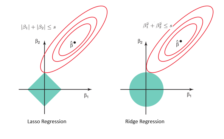
Source: https://online.stat.psu.edu/stat508/book/export/html/749
Considering the geometry of both the lasso (left) and ridge (right) models, the elliptical contours (red circles) are the cost functions for each. Relaxing the constraints introduced by the penalty factor leads to an increase in the constrained region (diamond, circle). Doing this continually, we will hit the center of the ellipse, where the results of both lasso and ridge models are similar to a linear regression model.
However, both methods determine coefficients by finding the first point where the elliptical contours hit the region of constraints. Since lasso regression takes a diamond shape in the plot for the constrained region, each time the elliptical regions intersect with these corners, at least one of the coefficients becomes zero. This is impossible in the ridge regression model as it forms a circular shape and therefore values can be shrunk close to zero, but never equal to zero.
Source: https://www.datacamp.com/tutorial/tutorial-lasso-ridge-regression
https://www.datacamp.com/datalab/w/e09a2743-6536-4d44-88e9-088be0edc682
SVC
# SVC
from sklearn.svm import SVC
from sklearn.model_selection import GridSearchCV
svc = SVC()
parameters = {'kernel': ['linear', 'rbf'],'C': [0.1, 1, 10]}
cv = GridSearchCV(svc, parameters, cv=5)
cv.fit(tr_features, tr_labels.values.ravel())
KNN
# KNN
# preprocessing
from sklearn import preprocessing
X = preprocessing.StandardScaler().fit(X).transform(X.astype(float))

from sklearn.model_selection import train_test_split
X_train, X_test, y_train, y_test = train_test_split( X, y, test_size=0.2, random_state=4)

# training
from sklearn.neighbors import KNeighborsClassifier
k = 4
neigh = KNeighborsClassifier(n_neighbors = k).fit(X_train,y_train)
neigh


# prediction
yhat = neigh.predict(X_test)

# evaluation
sklearn import metrics
print("Train set Accuracy: ", metrics.accuracy_score(y_train, neigh.predict(X_train)))
print("Test set Accuracy: ", metrics.accuracy_score(y_test, yhat))
# KNN example
from sklearn import neighbors, datasets, preprocessing
from sklearn.model_selection import train_test_split
from sklearn.metrics import accuracy_score

iris = datasets.load_iris()
X, y = iris.data[:, :2], iris.target
X_train, X_test, y_train, y_test = train_test_split(X, y, random_state=33)
scaler = preprocessing.StandardScaler().fit(X_train)
X_train = scaler.transform(X_train)
X_test = scaler.transform(X_test)

knn = neighbors.KNeighborsClassifier(n_neighbors=5)
knn.fit(X_train, y_train)

y_pred = knn.predict(X_test)
accuracy_score(y_test, y_pred)

output:
0.631578947368421
Feed forward artificial neural network
# multi-layer perceptron - classical feed forward artificial neural network
from sklearn.model_selection import GridSearchCV
from sklearn.neural_network import MLPClassifier
mlp = MLPClassifier()
parameters = {'hidden_layer_sizes': [(10,), (50,), (100,)],
     'activation': ['relu', 'tanh', 'logistic'],
     'learning_rate': ['constant', 'invscaling', 'adaptive']
}
cv = GridSearchCV(mlp, parameters, cv=5)
cv.fit(tr_features, tr_labels.values.ravel())
cv.best_estimator_
Random forest
“Random forests are applicable to a wide range of problems—you could say that they’re almost always the second-best algorithm for any shallow machine learning task. When the popular machine learning competition website Kaggle (http://kaggle.com) got started in 2010, random forests quickly became a favorite on the platform—until 2014, when gradient boosting machines took over. A gradient boosting machine, much like a random forest, is a machine learning technique based on ensembling weak prediction models, generally decision trees. It uses gradient boosting, a way to improve any machine learning model by iteratively training new models that specialize in addressing the weak points of the previous models. Applied to decision trees, the use of the gradient boosting technique results in models that strictly outperform random forests most of the time, while having similar properties. It may be one of the best, if not the best, algorithm for dealing with nonperceptual data today. Alongside deep learning, it’s one of the most commonly used techniques in Kaggle competitions. (from Chollet, 2017, Ch1)
# Random Forest - a collection of indepedent dection trees to improve
from sklearn.ensemble import RandomForestClassifier
from sklearn.model_selection import GridSearchCV
rf = RandomForestClassifier()
parameters = {
    'n_estimators': [5, 50, 250],
    'max_depth': [2, 4, 8, 16, 32, None]
}
cv = GridSearchCV(rf, parameters, cv=5)
cv.fit(tr_features, tr_labels.values.ravel())
Ensemble
# Ensemble - Boosting
from sklearn.ensemble import GradientBoostingClassifier
from sklearn.model_selection import GridSearchCV
gb = GradientBoostingClassifier()
parameters = {
    'n_estimators': [5, 50, 250, 500],
    'max_depth': [1, 3, 5, 7, 9],
    'learning_rate': [0.01, 0.1, 1, 10, 100]
}
cv = GridSearchCV(gb, parameters, cv=5)
cv.fit(tr_features, tr_labels.values.ravel())
Decision tree
# decision tree
Versitile algorithm, can perform both classification and regression tasks, also the
fundamental component of Random Forests, dont'require feature scaling or cetering
at all,


from sklearn.tree import DecisionTreeRegressor

# Split our data into a training and testing data
from sklearn.model_selection import train_test_split
X_train, X_test, Y_train, Y_test = train_test_split(X, Y, test_size=.2, random_state=1)

# training
model = DecisionTreeRegressor(criterion = 'mse')
model.fit(X_train, Y_train)
# evaluation / prediction
model.score(X_test, Y_test)
prediction = model.predict(X_test)
print("$",(prediction - Y_test).abs().mean()*1000)
from IPython.display import SVG
from graphviz import Source

graph = Source(tree.export_graphviz(model, out_file=None, feature_names=features))
SVG(graph.pipe(format='svg'))
K means
# K means - clustering
from sklearn.preprocessing import StandardScaler
scaler = StandardScaler()
customers_scaled = scaler.fit_transform(customers[['Income', 'SpendingScore']])

from sklearn.cluster import KMeans
km = KMeans(n_clusters = 3, n_init = 25, random_state = 1234)

km.labels_
km.inertia_
km.cluster_centers_

# determining k
wcss=[]; wcss.append(km.inertia_)
silhouette=[]; silhouette.append(silhouette_score(customers_scaled, km.labels_))
calinski=[]; calinski.append(calinski_harabasz_score(customers_scaled, km.labels_))
PCA
Semi-supervised
