Contents
Resources
Commands

where python
whereis python
idle
py -V
py -3 --version

Linux CTL
ls -l
ls -lha
ls -lh
clear
ls
dir
cd
pwd

conda
conda init
where conda
conda -V
conda list

conda env list
conda info --envs

conda create -n yourenvname python=x.x anaconda
conda create -p C:\Apps\Anaconda3\envs\yourenvname python==3.10.11
conda activate C:\Apps\Anaconda3\envs\yourenvname
pip install -r "<Folder>\requirements.txt"
pip3 list

python -m venv yourenvname
cd yourenvname
source bin/activate
deactivate

py -m pip install --upgrade pip

# to update Spyder kernels, open conda shell
(base) C:\Users\hy11>conda install spyder‑kernels=2.1
(base) C:\Users\hy11>pip install spyder‑kernels==2.1.*

#create the venv
pip install yourenvname
python -m venv yourenvname
yourenvname\Scripts\activate
deactivate

# If your virtual environment is in a directory called 'venv':
rm -r venv

pip install jupyter

pip install nbconvert

jupyter nbconvert testnotebook*.ipynb --to python
jupyter nbconvert testnotebook.ipynb --to script
jupyter nbconvert testnotebook.ipynb testnotebook1.ipynb testnotebook2.ipynb --to python
To save Korean characters (Hangul) correctly in an Excel CSV file, follow these steps:

1. Save CSV with UTF-8 Encoding
Korean characters require UTF-8 encoding to be displayed properly in CSV files. Here’s how you can do it:

Using Excel (Windows)
Enter your data in Excel.
Click File → Save As.
Choose CSV UTF-8 (Comma delimited) (*.csv) from the file format dropdown.
Click Save.

Open the CSV in Excel Correctly
If you experience encoding issues when opening in Excel:

Open Excel and go to Data → Get External Data → From Text.
Select your .csv file.
Choose 65001: Unicode (UTF-8) as the file origin.
Click Next and follow the steps to import.


import pandas as pd

# Sample data with Korean characters
data = {'이름': ['김철수', '박영희'], '나이': [25, 30], '도시': ['서울', '부산']}

# Create a DataFrame
df = pd.DataFrame(data)

# Save as CSV with UTF-8 encoding
df.to_csv('korean_data.csv', index=False, encoding='utf-8-sig')

To install Hagul font in Colab
!apt-get update
!apt-get install -y fonts-nanum

# Define a Korean font path (use NanumGothic or Malgun Gothic)
font_path = "/usr/share/fonts/truetype/nanum/NanumGothic.ttf"  # Linux/macOS (install if needed)

import os
os.listdir('/usr/share/fonts/truetype/nanum')

import matplotlib.font_manager as fm # Import the font_manager module

# Korean font setup
font_path = "/usr/share/fonts/truetype/nanum/NanumGothic.ttf"  # Linux/macOS

# Confirm font existence
if not os.path.isfile(font_path):
    print(f"Font not found at {font_path}. Please install or correct the path.")
    font_path = None
    font_prop = None
else:
    font_prop = fm.FontProperties(fname=font_path)
    print(f"Font found at {font_path}.")

# Generate Word Cloud with Korean font, handle font_path being None wordcloud = WordCloud(
        width=800,
        height=400,
        background_color="white",
        font_path=font_path  # Use the specified or default font
).generate(text)
WRDS
Important: The WRDS Cloud compute nodes (wrds-sas1, wrds-sas36, etc) are not Internet-accessible. So you must use the two WRDS Cloud head nodes (wrds-cloud-login1-h or wrds-cloud-login2-h) to upload packages to your WRDS home directory. Once uploaded, however, you can use them on the WRDS Cloud compute nodes as normal. https://wrds-www.wharton.upenn.edu/pages/support/the-wrds-cloud/using-ssh-connect-wrds-cloud
WRDS offers Jupyter hub in its cloud with Linux machine and theoretically it will be faster and can lengthen the runtime. This is its main benefit. However, some details are required.
Jupyter terminal does not outbound connectivity to the internet so you cannot create a virtual environment in this way.
Instead, you need to access the log-in node using Putty SSH connection. https://wrds-www.wharton.upenn.edu/pages/support/the-wrds-cloud/using-ssh-connect-wrds-cloud
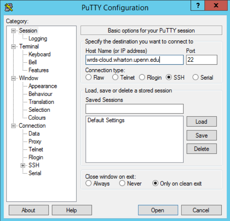
need to open putty app<br>
log in
wrds-cloud.wharton.upenn.edu <br>
use log in id and password to sign on<br>
create a virtual env diredctory<br>
using <br>python3 -m venv --copies ~/virtualenv <br>
Activate the virtualenv: <br>source ~/virtualenv/bin/activate <br>
and install the desired packages<br>
you are on a login node and your virtual environment is activated,
You can install your packages. You must also install the ipykernel package.
Once you have installed your packages and Jupyter, you must create a custom Jupyter kernel. Do this by running the following command and giving it a name, remembering this name for later use: <br>
pip install ipykernel
python3 -m ipykernel install --user --name=<kernel_name>\
pip install -r "<Tidy-Finance-with-Python Folder>\requirements.txt"
Log in to JupyterHub and start a JupyterLab instance. Click the “+” in the upper left-hand corner to start a new launcher. In the first row of the launcher tab, “Notebooks,” you will see a new kernel with the name you gave your kernel. Click it to start a notebook. This notebook uses the virtual environment you set up, including the packages you installed. Notice under “Notebook” and “Console” that there are several kernels, including the one named my-jupyter-env. Launching this will use the virtual environment from which you created the kernel. https://wrds-www.wharton.upenn.edu/pages/support/programming-wrds/programming-python/installing-your-own-python-packages/#introduction
Google Colab Pro
Google Colab is a web-based iPython Notebook service for interactive coding. Google Colab offers free access to Nvidia K80 GPU, and it is becoming a popular tool for quick prototyping and visualization. Colab is easy to learn and it is very similar to Jupyter Notebook, another very popular tool for interactive coding.
https://colab.research.google.com/notebooks/pro.ipynb#scrollTo=SKQ4bH7qMGrA
https://colab.research.google.com/drive/1YKHHLSlG-B9Ez2-zf-YFxXTVgfC_Aqtt#scrollTo=pmECBCuVdu8N
https://colab.research.google.com/notebooks/intro.ipynb#
https://colab.research.google.com/notebooks/
Python Tutorial With Google Colab https://colab.research.google.com/github/cs231n/cs231n.github.io/blob/master/python-colab.ipynb
Overview of Colaboratory Features: https://colab.research.google.com/notebooks/basic_features_overview.ipynb
https://colab.research.google.com/github/Hvass-Labs/TensorFlow-Tutorials/blob/master/01_Simple_Linear_Model.ipynb
Introduction to Colab and Python: https://colab.research.google.com/github/tensorflow/examples/blob/master/courses/udacity_intro_to_tensorflow_for_deep_learning/l01c01_introduction_to_colab_and_python.ipynb#scrollTo=YHI3vyhv5p85
External data: Local Files, Drive, Sheets, and Cloud Storage: https://colab.research.google.com/notebooks/io.ipynb
Faster GPUs
Users who have purchased one of Colab's paid plans have access to premium GPUs. You can upgrade your notebook's GPU settings in Runtime > Change runtime type in the menu to enable Premium accelerator. Subject to availability, selecting a premium GPU may grant you access to a V100 or A100 Nvidia GPU.

The free-of-charge version of Colab grants access to Nvidia's T4 GPUs subject to quota restrictions and availability.

You can see what GPU you've been assigned at any time by executing the following cell. If the execution result of running the code cell below is "Not connected to a GPU", you can change the runtime by going to Runtime > Change runtime type in the menu to enable a GPU accelerator, and then re-execute the code cell.

More memory
Users who have purchased one of Colab's paid plans have access to high-memory VMs when they are available. You can see how much memory you have available at any time by running the following code cell. If the execution result of running the code cell below is "Not using a high-RAM runtime", then you can enable a high-RAM runtime via Runtime > Change runtime type in the menu. Then select High-RAM in the Runtime shape dropdown. After, re-execute the code cell.

Longer runtimes
Background execution
Connecting to a local hard drive within Google Colab
One nice feature of Colab is that you can connect a local Andaconda Python engine so that you can easily access local data and write to a local drive. However, it is a little tricky to connect locally. The default in Colab is to connect globally, but you can still change its setting to connect locally in Google Colab.

Open Anaconda Powershell prompt, and then execute the following command:

jupyter notebook --NotebookApp.allow_origin='https://colab.research.google.com' \

and scroll down to find the token and then copy & paste token and execute. This is tricky because you will get an Error when connecting to local Jupyter to use Googel Colab. See below:
When connecting to local runtime from Google Colab, I had no problem from Step 1-3. But when I copy & pasted the URL to the connect prompt window, I kept getting the following message "Blocking Cross Origin API request for /http_over_websocket" in Anaconda Prompt. I googled and found the solution that worked for me. All I had to do was to type the following command in my Anaconda Prompt. After this, I had no issue connecting to local runtime.

jupyter notebook --NotebookApp.allow_origin='https://colab.research.google.com' \
  --port=8888 --no-browser

type one below only ------ this is working

jupyter notebook --NotebookApp.allow_origin='https://colab.research.google.com' \

For details, see this thread: https://github.com/googlecolab/jupyter_http_over_ws/issues/1#issuecomment-387879322
This is a shell command, I remember.....
Google instruction -- not working
pip install jupyter_http_over_ws jupyter serverextension enable --py jupyter_http_over_ws

this one is also not working either
jupyter notebook \ --NotebookApp.allow_origin='https://colab.research.google.com' \ --port=8888 \ --NotebookApp.port_retries=0

Ad then after not working troubleshoot says this but still not working
pip install --upgrade jupyter_http_over_ws>=0.0.7 && \ jupyter serverextension enable --py jupyter_http_over_ws

However, Slack says that this one is working and it did work:
jupyter notebook --NotebookApp.allow_origin='https://colab.research.google.com' \ --port=8888 --no-browser
Set-ups
from IPython.core.interactiveshell import InteractiveShell
InteractiveShell.ast_node_interactivity = "all"

from google.colab import drive
drive.mount('/content/drive')

You can use %%capture to prevent output from cluttering your notebook, especially if a cell produces a lot of text or warnings that you don't need to see.
%%capture # or
-q   # as quiet
Change Directory (os.chdir)
- Purpose: Changes the current working directory to the specified path.
- Effect: All subsequent file operations (like opening files) will be relative to this new directory.
- Example:
import os os.chdir('/path/to/directory')After this command, if you open a file with a relative path, it will look in/path/to/directory.
Append Directory (sys.path.append)
- Purpose: Adds a directory to the list of paths that Python searches for modules.
- Effect: Allows you to import modules from the specified directory.
- Example:
import sys sys.path.append('/path/to/directory')After this command, you can import modules located in/path/to/directoryas if they were in the standard library or current working directory.
Key Differences
Use Case: Use os.chdir when you need to work with files in a different directory. Use sys.path.append when you need to import modules from a non-standard directory.
Scope: os.chdir affects the working directory for the entire script, while sys.path.append only affects module import paths.
Part I: Setting Up Your Environment
A solid setup is the foundation for mastering Python. In this section, we will walk through installing Miniconda, creating virtual environments, configuring Visual Studio Code (VSCode), integrating GitHub Copilot for AI-powered code suggestions, and exploring AI tools for assistance.

1. Install Miniconda
Why Miniconda?
Miniconda is a very lightweight version of Anaconda, containing only Python and the Conda package manager. It simplifies library installation, ensuring each project has the right packages (no more “dependency nightmares”). Alternatively, you can use Anaconda, a full-featured distribution with more pre-installed libraries -- though it's more of a hassle to manage in the long term. Both are excellent ways to use python.

Windows
Download Miniconda.
Run the installer, accept defaults.
Open Anaconda Prompt, type
conda --version to confirm.

Mac
Download Miniconda.
In Terminal, navigate to your Downloads folder with cd Downloads.
Run bash Miniconda3*.sh and follow the prompts.
Type
conda --version to verify the installation.
for alternatives and more detailed instructions, refer to the official install instructions for Miniconda

Quick Check
OS	Download Link	Verify Command
Windows	Miniconda	conda --version (Anaconda Prompt)
Mac	Miniconda	conda --version (Terminal)

2. Create Virtual Environments
Why Virtual Environments?
Virtual environments keep each project’s libraries neatly separated, preventing conflicts among different assignments. Note that we use python 3.12 -- the newest version at the time of writing is 3.13; however, it is not yet supported by all libraries, least of not the ones that are used in finance. They will eventually update, but you can think of 3.12.x as the most stable version for now.

Open Anaconda Prompt (Windows) or Terminal (Mac).
note: you can replace investment_env with any name you like, but it is recommended to use a name that is relevant to the project you are working on -- we will be using investment_envfor example going forward

Create an environment:
conda create -n investment_env python=3.12
(Type y when prompted.)

Activate it:
conda activate investment_env

Install useful packages:
note: you can install more packages as needed, but these are the most common ones used in finance, additionally, conda and pip are both, and occationally one is better than the other, so it is recommended to know how to use both. I personally default to pip when able.

conda install pandas
pip install yfinance

Deactivate when done:
conda deactivate

Handy Commands
Command	Purpose
conda create -n name python=3.12	Creates a new environment
conda activate name	Switches to the environment
conda install package_name	Installs a package via Conda
pip install package_name	Installs a package via pip
conda deactivate	Exits the environment

3. Configure VSCode with Python & Jupyter
Why VSCode?
Visual Studio Code is a free, powerful editor, perfect for coding and running Jupyter notebooks—essential for data manipulation and visualization in finance.

This one may be a bit more complicated, but it is worth it. VSCode is a very powerful tool that can be used for many different things, and it is very useful for coding in python. If this is too much, I recommend Google's Colab, which is a free online Jupyter notebook that is far easier to use than most other options and is free.

Download VSCode.
Open VSCode, go to Extensions (Ctrl + Shift + X), and install:
Python
Jupyter
Select your Python environment:
Command Palette (Ctrl + Shift + P) → “Python: Select Interpreter” → Pick investment_env.
Create a new Jupyter notebook:
Command Palette → “Jupyter: Create New Notebook” → Start coding interactively.

4. Get GitHub Student & Copilot
what is GitHub? GitHub is a platform where developers can store, share, and collaborate on code. It is a very useful tool for students and professionals alike, and it is a great way to show off your work to potential employers -- it's additionally ubiquitous in the tech/finance industry, so it is a good idea to get familiar with it.

Why GitHub Student?
Signing up for the GitHub Student Developer Pack grants you GitHub Pro and free access to Copilot, an AI tool that suggests code as you type. This is an extremely useful tool that can save you a lot of time and effort at the early stages of learning, and it is free for students.

Go to GitHub Education and apply using your student credentials. (Follow the instructions carefully -- I used the top section of my degree audit as proof and put texas state graduate student in my github bio.)
After approval, open VSCode → Extensions → Install Copilot.
Sign in with GitHub to enable AI-powered code completions.
Benefits at a Glance
Feature	Free GitHub	Student (Pro)
Private Repos	Limited	Unlimited
Copilot Integration	No	Yes
Team Collaboration	Basic	Enhanced

5. Explore AI Tools
Why AI Tools?
Tools like Perplexity, ChatGPT, Grok, and Claude can speed up coding tasks, answer questions, and inspire new approaches. Always verify their outputs, as AI can occasionally err.

Perplexity: Research with citations (Link)
ChatGPT: Versatile chatbot (Link)
Grok: Specialized code assistance (Link)
Claude: General AI assistant (Link)
Use them to ask questions like “How do I calculate Sharpe ratios in Python?” or “Show me an example of mean-variance portfolio optimization.” Then refine and confirm with official documentation.

Tool Snapshot
Tool	Best For	Free Access?
Perplexity	Research with sources	Yes
ChatGPT	Code & explanations	Yes
Grok	Code refactoring	Yes
Claude	General AI help	Yes
response = requests.get('https://api.github.com')
print(response.status_code)  # HTTP status code
print(response.text)         # Response content as text

if response.status_code == 200:
    print("Success!")
elif response.status_code == 404:
    print("Not Found.")

>>> import requests

>>> response = requests.get("https://api.github.com")
>>> response.content
b'{"current_user_url":"https://api.github.com/user", ...}'

>>> type(response.content)
<class 'bytes'>

>>> response.text
'{"current_user_url":"https://api.github.com/user", ...}'

>>> type(response.text)
<class 'str'>

>>> response.encoding = "utf-8"  # Optional: Requests infers this.
>>> response.text
'{"current_user_url":"https://api.github.com/user", ...}'

>>> response.json()
{'current_user_url': 'https://api.github.com/user', ...}

>>> type(response.json())
<class 'dict'>

>>> response_dict = response.json()
>>> response_dict["emojis_url"]
'https://api.github.com/emojis'

>>> import requests

>>> response = requests.get("https://api.github.com")
>>> response.headers
{'Server': 'GitHub.com',
...
'X-GitHub-Request-Id': 'AE83:3F40:2151C46:438A840:65C38178'}
Python’s Pickle module is a popular format used to serialize and deserialize data types.
pickle.dump converts Python objects into a byte stream that can be saved to files and later reconstructed. This process is called serialization, making it crucial for data storage and transfer.
import pickle

data = {'name': 'John', 'age': 30, 'city': 'New York'}

# Saving to a file
with open('data.pkl', 'wb') as file:
    pickle.dump(data, file)

In Python, we work with high-level data structures such as lists, tuples, and sets. However, when we want to store these objects in memory, they need to be converted into a sequence of bytes that the computer can understand. This process is called serialization.
The next time we want to access the same data structure, this sequence of bytes must be converted back into the high-level object in a process known as deserialization.
Unlike serialization formats like JSON, which cannot handle tuples and datetime objects, Pickle can serialize almost every commonly used built-in Python data type. It also retains the exact state of the object which JSON cannot do.
`apt` is a package management tool used in Debian-based Linux distributions, such as Ubuntu. It stands for **Advanced Package Tool** and is used to install, update, and remove software packages.

  !sudo apt update
  This command updates the list of available packages and their versions.

  !sudo apt install package_name
  This installs the specified package.

  !sudo apt remove package_name
  This removes the specified package.

Usage in Jupyter Notebooks: In environments like Jupyter notebooks or Google Colab, you can use `!apt` to run these commands directly from the notebook interface.

The `sudo` command in Unix-like operating systems allows a permitted user to execute a command as the superuser or another user, as specified by the security policy. The name `sudo` stands for "superuser do," reflecting its primary function.

### Key Features
- **Elevated Privileges**: `sudo` temporarily grants administrative privileges to perform tasks that require higher permissions.
- **Security**: Users authenticate with their own password, not the superuser's, reducing the risk of compromising the superuser's credentials.
- **Granular Control**: The `/etc/sudoers` file allows administrators to define which users can run specific commands as `sudo` and under what conditions.

### Example Usage
- **Running a Command with Elevated Privileges**:
  sudo apt-get update
  This command updates the package lists with administrative privileges.

- **Editing a System File**:
  sudo nano /etc/hosts
  This opens the `/etc/hosts` file in the `nano` editor with the necessary permissions to modify it.

### Benefits
- **Convenience**: Users can perform administrative tasks without logging in as the root user.
- **Auditability**: Actions performed with `sudo` are logged, providing a record of who did what and when.
import pkg_resources
import pip
import sys
installedPackages = {pkg.key for pkg in pkg_resources.working_set}
required = {'nltk', 'spacy', 'textblob','gensim'}
missing = required - installedPackages
if missing:
!pip install nltk==3.4
!pip install textblob==0.15.3
!pip install gensim==3.8.2
!pip install -U SpaCy==2.2.0
!python -m spacy download en_core_web_lg
!pip install pandas==2.2.1  # restart the session
!pip install pyarrow
# Jupyter uses forward slashes to access folders in path. For example.,
path = 'C:/Users/hy11/Documents/......../data/facebook.csv'
# or path = 'C:\\Users\\hy11\\Documents\\........\\data\\facebook.csv'
help(sum)

import warnings
warnings.filterwarnings('ignore')

import pandas as pd
pd.options.mode.chained_assignment = None # default='warn'
numpy.inf
IEEE 754 floating point representation of (positive) infinity.
import numpy as np
np.set_printoptions(precision = 2)

import pandas as pd
pd.set_option('max_rows', 20)
pd.options.display.max_rows = 100
pd.options.display.float_format = '{:,.2f}'.format
# How to see more data
with pd.option_context('display.min_rows', 30, 'display.max_columns', 82):
   display( df.query('`ColumnA`.isna()'))
from google.colab import files
uploaded = files.upload()

import os
directory_path = path

# List comprehension to find all PDF files
pdf_files = [file for file in os.listdir(directory_path) if file.lower().endswith('.pdf')]

print("PDF files found:", pdf_files)
import os
import openai
from openai import OpenAI
from google.colab import userdata

os.environ["OPENAI_API_KEY"] = userdata.get('OPENAI_API_KEY')
import os
os.chdir('/content/drive/My Drive/Colab Notebooks/data/')
os.getcwd()
os.listdir()

list = os.listdir()
number_files = len(list)
print(number_files)
!pip install https://github.com/pandas-profiling/pandas-profiling/archive/master.zip

# Restart the kernel

import pandas as pd
from pandas_profiling import ProfileReport
profile = ProfileReport(df, title=’Heart Disease’, html={‘style’:{‘full_width’:True}})
profile.to_notebook_iframe()
Magic commands
%time: Time the execution of a single statement

%timeit: Time repeated execution of a single statement for more accuracy

%prun: Run code with the profiler

%lprun: Run code with the line-by-line profiler

%memit: Measure the memory use of a single statement

%mprun: Run code with the line-by-line memory profiler

%cd Change the current working directory.
%conda Run the conda package manager within the current kernel.

%dirs Return the current directory stack.

%load_ext Load an IPython extension by its module name.

%pwd Return the current working directory path.
IN: name = input("What is your name?")
OUT: What is your name?

IN: type (7)
OUT: int

IN: type("dog")
OUT: str

IN: min(36, 34, 45)
OUT: 34

IN: Grade = 85
    If Grade >= 60:
       print("Passed")
    elif Grade <= 50:
       print("Failed")
    else
       print("Retake")
OUT: Passed

IN: P = 3
    N = 0

    while P <= 50:
        P = P * 3
        N  +=

    P
OUT: 81

IN: total = 0

    for number in [2, -3, 0, 17, 9]
        total += number

    total
OUT: 25

IN: for counter in range(11):
        print(counter, end=' ')
OUT: 0 1 2 3 4 5 6 7 8 9 10
IN: print (10, 20, 30, sep=",")
OUT: 10,20,30

IN: total = 0
    grade_counter = 0
    grades = [98, 76, 71, 87, 83, 90, 57, 79, 82, 94]

    for grade in grades:
        total += grade
        grade_counter += 1

    average = total/grade_counter
    print(f'class average is {average}')
OUT: Class average is 81.7

IN: for number in range(0, 10, 2):
    print(number, end = "  ")
OUT: 0 2 4 6 8

IN: grade = 87

    if grade != -1:
       print("The next grade is", grade)
OUT: The next grade is 87

IN: import statistics
    grades = [85, 93, 45, 89, 85]
    sum(grades/len(grades))
OUT: 79.4
IN: statistics.mean(grades)
OUT: 79.4
IN: Statistics.median(grades)
OUT: 85
IN: sorted(grades)
OUT:[45, 85, 85, 89, 93]

IN: def square(number):
        return number ** 2
    square(10)
OUT: 100

IN: print('The Square of 10 is ', square(10))
OUT: The Square of 10 is 100.

IN: import math
    from math import ceil,floor
    ceil(9.5)
OUT: 10

IN: import math
    math.pow(2.0, 7.0)
OUT: 128

IN: c = [1, 2, 3, 4, 5]
    len(c)
OUT: 5
IN: c[0]=0
    c
OUT: [0, 2, 3, 4, 5]

IN: a_list =[]
    for number in range (1, 7):
        a_list += [number]
    a_list
OUT: [1, 2, 3, 4, 5, 6]

IN: list1 = [1, 2, 3]
    list2 = [40, 50]
    concatenated_list = list1 + list2
    concatenated_list
OUT: [1, 2, 3, 40, 50]

IN: for i in range(len(concatenated_list)):
        print(f'{i} = {concatenated_list[i]}')
OUT: 0 = 1
     1 = 2
     2 = 3
     3 = 40
     4 = 50

IN: tuple = (6, 5, 4)
    tuple[0] * 2 + tuple[1] * 2 + tuple[3] * 2
OUT: 30

IN: colors = ['red', 'blue', 'green']
    for index, value in enumerate(colors):
        print(f'{index}:{value}')
OUT: 0:red
     1:blue
     2:green

IN: def modify_elements(items):
        for i in range(len(items)):
            items[i] *= 2
    numbers = [10, 3, 7, 1, 9]
    modify_elements(numbers)
    numbers
OUT: [20, 6, 14, 2, 18]

IN: numbers.sort()
OUT: [2, 6, 14, 18, 20]

IN: numbers.sort(reverse = True)
OUT: [20, 18, 14, 6, 2]
pip install pandas_datareader  *** to install pandas
pip install fix_yahoo_finance  *** to install yahoo finance? won't work
pip install yfinance --upgrade --no-cache-dir  ***instead use this one
pip install --upgrade pip
## from https://aroussi.com/post/python-yahoo-finance

IN: import pandas as pd
    import matplotlib.pyplot as plt
OUT:

IN: from pandas_datareader import data as pdr
    import yfinance as yf
    yf.pdr_override()
    data = pdr.get_data_yahoo("SPY", start="2017-01-01", end="2017-04-30")
OUT: [*********************100%***********************]  1 of 1 downloaded

IN:print (data.head())
OUT: ## it will show head

IN: def plot_data(A, title = 'His Price'):
    ax = A.plot (fontsize = 12)
    plt.show()
    plot_data(data['Adj Close'])
OUT: ## it will show the graph
###########################################################33
IN: def returns(B):
OUT:
Tuple, List, Dictionary
list = [1, 2, 3, 4]
len(list)
output:
4number_list = [2,4,6,8,10,12]
print(number_list[::2])
output:
[2, 6, 10]
pets = ['dogs', 'cat', 'bird']
pets.append('lizard')
pets
output:
['dogs', 'cat', 'bird', 'lizard']
person = {'name': 'fred', 'age': 29}
print(person['name'], person['age'])
output:
fred 29
dict_1 = {'apple':3, 'oragne':4, 'pear':2}
dict_1
output:
{'apple': 3, 'oragne': 4, 'pear': 2}
dict_1['apple']
output:
3
dict_1.keys()
output:
dict_keys(['apple', 'oragne', 'pear'])
dict_1.values()
output:
dict_values([3, 4, 2])
cities_to_temps = {"Paris": 28, "London": 22, "Seville": 36, "Wellesley": 29}
for key, value in cities_to_temps.items():
print(f"In {key}, the temperature is {value} degrees C today.")
output:
In Paris, the temperature is 28 degrees C today.
In London, the temperature is 22 degrees C today.
In Seville, the temperature is 36 degrees C today.
In Wellesley, the temperature is 29 degrees C today.
print('Hello ' + 'World')
Hello World

apples = 'apples'
print('I have', 2, apples)
I have 2 apples
Datetime
# from string to datetime or date
from datetime import datetime
datetime.strptime('2009-01-01', '%Y-%m-%d')

output:
datetime.datetime(2009, 1, 1)

datetime.strptime('2009-01-01', '%Y-%m-%d').date()

Output:
datetime.date(2009, 1, 1)
I/O
The tarfile module makes it possible to read and write tar archives, including those
using gzip, bz2 and lzma compression.
Use the zipfile module to read or write .zip  files, or the higher-level functions
in shutil.

import tarfile
tar = tarfile.open("sample.tar.gz")
tar.extractall(filter='data')
tar.close()
The urllib.request module defines functions and classes which help in opening URLs
(mostly HTTP) in a complex world — basic and digest authentication, redirections,
cookies and more.
urllib is part of the Python Standard Library and offers basic functionality for
working with URLs and HTTP requests.
urllib3 is a third-party library that provides a more extensive feature set for
making HTTP requests and is suitable for more complex web interaction tasks.
It must be installed separately.

import urllib.request
with urllib.request.urlopen('http://www.python.org/') as f:
     print(f.read(300))
import urllib.request
min_date = '1963-07-31'
max_date = '2020-03-01'

ff_url = 'https://mba.tuck.dartmouth.edu/pages/faculty/ken.french/ftp/F-F_Research_Data_5_Factors_2x3_CSV.zip'
urllib.request.urlretrieve(ff_url, 'factors.zip')
!unzip -a factors.zip
!rm factors.zip
with open('text.txt') as f:
     text_in = f.read()

print(text_in)

with open(os.path.join(data_path, 'text_sample.txt'), 'r', encoding='utf-8') as file:
    file_content = file.read()
print(file_content)
output:
Learning Python is great.
Good luck!
import pandas as pd
url = 'https://github.com/mattharrison/datasets/raw/master/data/ames-housing-dataset.zip'
df = pd.read_csv(url, engine='pyarrow', dtype_backend='pyarrow')
#removing the file.
os.remove("file_name.txt")

file_name = "python.txt"
os.rename(file_name,'Python1.txt')
# to tell the path
import sys
sys.path.append('/content/drive/My Drive/Colab Notebooks/data/')
import sys
print(sys.version)

#Listing out all the paths
import sys
print(sys.path)

# print out all modules imported
sys.modules"
print ('%s is %d years old' % ('Joe', 42))

Output:
Joe is 42 years old
print('We are the {} who say "{}!"'.format('knights', 'Ni'))

Output:
We are the knights who say "Ni!"
Data Wrangling – Numpy / Pandas
np.random.seed(42)

Setting the random seed is important for reproducibility.
By fixing the seed to a specific value (in this case, 42),
you ensure that the sequence of random numbers generated
by NumPy will be the same every time you run your code,
assuming that other sources of randomness in your code are
also controlled or fixed.
X_b = np.c_[np.ones((100, 1)), X] # add x0 = 1 to each instance
>>> np.ones(5)
array([1., 1., 1., 1., 1.])
>>> np.ones((2, 1))
array([[1.],
       [1.]])
>>> np.c_[np.array([1,2,3]), np.array([4,5,6])]
array([[1, 4],
       [2, 5],
       [3, 6]])
# data type conversion
df['year'].astype(str)
df['number'].astype(float)

y = y.astype(np.uint8)
# We can alternatively use glob as this directly allows to include pathname matching.
# For example if we only want Excel .xlsx files:

data_path = os.path.join(os.getcwd(), 'data_folder')

from glob import glob
glob(os.path.join(data_path, '*.xlsx'))

output:

'/content/drive/MyDrive/Colab Notebooks/data/output.xlsx',
'/content/drive/MyDrive/Colab Notebooks/data/beta_file.xlsx',
# index
df = df.set_index("Column 1")

df.index.name = "New Index"

# making data frame from csv file
data = pd.read_csv("nba.csv", index_col ="Name")

# remove own index with default index
df.reset_index(inplace = True, drop = True)
# to rename
data.rename(columns={'OLD': 'NEW'}, inplace=True)

# reformat column namess
df.columns = df.columns.str.lower().str.replace(" ", "_")
df["column_name"].str.lower()

# to print memory usage
memory_per_column = df.memory_usage(deep=True) / 1024 ** 2

df_cat = df.copy()
Slices can be passed by name using
.loc[startrow:stoprow:step, startcolumn:stopcolumn:step]

or by position using .iloc[start:stop:step, start:stop:step].

df.loc[2::10, "name":"gender"]
.isna()
.notna()

Always use pd.isnull() or pd.notnull() when conditioning on missing values.
This is the most reliable.

df[pd.isnull(df['Column1'])
df[pd.notnull(df['Column2'])].head()

df.query('ColumnA'.isna())
try:
     df = pd.read_csv(url, skiprows=0, header=0)
     print("Data loaded successfully.")
except Exception:
     print("Error loading sheet")
     # If an error occurs, halt further execution
     raise
if __name__ == "__main__":
     main()
# use the break and continue statements
for x in range(5,10):
    if (x == 7): break
    if (x % 2 == 0): continue
    print (x)
pd.concat([data_FM.head(), data_FM.tail()])
pd.concat([df.head(10), df.tail(10)])
# Categoricals - Pandas 2
df.select_dtypes('string')  # or 'strings[pyarrow]'
# Categoricals
df.select_dtypes('string').describe().T
What is type and dtype in Python?

The type of a NumPy array is numpy.ndarray ; this is just the type of Python object

it is (similar to how type("hello") is str for example). dtype just defines how bytes

in memory will be interpreted by a scalar (i.e. a single number) or an array and

the way in which the bytes will be treated (e.g. int / float ).
# Convert string columns to the `'category'` data type to save memory.
(df
.select_dtypes('string')
.memory_usage(deep=True)
.sum()
)


(df
.select_dtypes('string')
.astype('category')
.memory_usage(deep=True)
.sum()
)
# Missing numeric columns (and strings in Pandas 1)

df.isna().mean().mul(100).pipe(lambda ser: ser[ser > 0])
# sample five rows
df.sample(5)
# LAMBDA
adult_data['Label'] = adult_data['Salary'].map(lambda x : 1 if '>50K' in x else 0)
df.assign(Total_Salary = lambda x: df['Salary'] + df['Bonus'])
# SORT_VALUES
oo.sort_values(by = ['Edition', 'Athlete'])

# Count unique values
oo['NOC].value_counts(ascending = True) oo['NOC].unique()
oo[(oo['Medal']=='Gold') & (oo['Gender'] == 'Women')]
oo[oo['Athlete'] == 'PHELPS, Michael']['Event']
oo["Athlete"].value_counts().sort_values(ascending = False).head(10)
df['Label'].value_counts().plot(kind='bar') # or df.groupby('Label').size().plot(kind='bar')
oo[oo.Athlete == 'PHELPS, Michael'][['Event', 'City','Edition']]  #or oo[oo['Athlete'] == 'PHELPS, Michael'][['Event', 'City','Edition']]
# Delete a single column from the DataFrame
data = data.drop(labels="deathes", axis=1)

# Delete multiple columns from the DataFrame
data = data.drop(labels=["deaths", "deaths_per_million"], axis=1)

# Note that the "labels" parameter is by default the first, so # the above lines can be written slightly more concisely:
data = data.drop("deaths", axis=1)
data = data.drop(["deaths", "deaths_per_million"], axis=1)

# Delete a single named column from the DataFrame
data = data.drop(columns="cases")

# Delete multiple named columns from the DataFrame
data = data.drop(columns=["cases", "cases_per_million"])
pd.concat([s1, s2], axis=1)
pd.concat([s1, s2], axis=1).reset_index() a.to_frame().join(b)

# Delete column numbers 1, 2 and 5 from the DataFrame # Create a list of all column numbers to keep
columns_to_keep = [x for x in range(data.shape[1]) if x not in [1,2,5]]

# Delete columns by column number using iloc selection
data = data.iloc[:, columns_to_keep]

# delete a single row by index value 0
 data = data.drop(labels=0, axis=0)

# delete a few specified rows at index values 0, 15, 20.
# Note that the index values do not always align to row numbers.
data = data.drop(labels=[1,15,20], axis=0)

# delete a range of rows - index values 10-20
data = data.drop(labels=range(40, 45), axis=0)

# The labels parameter name can be omitted, and axis is 0 by default
# Shorter versions of the above:
data = data.drop(0)
data = data.drop([0, 15, 20])
data = data.drop(range(10, 20))
data.shape
output: (238, 11)

# Delete everything but the first 99 rows.
data = data[:100]
data.shape
output: (100, 11)

ata = data[10:20]
data.shape
output: (10, 11)
# divide multiple columns by a number efficiently
df_ff[['MKT_RF','SMB','HML','RMW','CMA','RF']] /= 100.0
# handling missing variables
df = df.append(another_row)
.loc .iloc
loc: Accesses data by labels (row names and column names). It is inclusive of both the start and stop bounds.
iloc: Accesses data by integer position (row and column indices). It is inclusive of the start bound but exclusive of the stop bound.

loc gets rows (and/or columns) with particular labels.
iloc gets rows (and/or columns) at integer locations.

import pandas as pd

colors = pd.Series(
    ["red", "purple", "blue", "green", "yellow"],
    index=["a", "b", "c", "d", "e"]
)
print(colors)

print()
print("Using iloc:", colors.iloc[2])
print("Using loc:", colors.loc["d"])

output:
a       red
b    purple
c      blue
d     green
e    yellow
dtype: object

Using iloc: blue
Using loc: green

data_ml.loc[data_ml["R12M_Usd"] > 50, ["stock_id", "date", "R12M_Usd"]]

df.dtypes
df.shape
df.iloc[3:5]
df.loc[(df["Col_A"] == "brown") & (df["Col_B"] == "blue"), ["Col_D", "Col_Z"]]
Lamda
def add(x, y):
    return x + y

This is the same as

add = lambda x, y: x + y
print(add(3, 5))

Output:
8

# LAMBDA
adult_data['Label'] = adult_data['Salary'].map(lambda x : 1 if '>50K' in x else 0)
df.assign(Total_Salary = lambda x: df['Salary'] + df['Bonus'])
(lambda x, y: x * y)(3,4)

Output:
12

str1 = 'Texas'
reverse_upper = lambda string: string.upper()[::-1]
print(reverse_upper(str1))

Output:
SAXET

is_even_list = [lambda arg=x: arg * 10 for x in range(1, 5)]

for item in is_even_list:
    print(item())

Output:
10
20
30
40

>>> (lambda x: x + 1)(2)
3

list1 = ["1", "2", "9", "0", "-1", "-2"]
# sort list[str] numerically using sorted()
# and custom sorting key using lambda

print("Sorted numerically:", sorted(list1, key=lambda x: int(x)))

Output:
Sorted numerically: ['-2', '-1', '0', '1', '2', '9']

import pandas as pd
df = pd.DataFrame({'col1': [1, 2, 3, 4, 5], 'col2': [0, 0, 0, 0, 0]})
print(df)
df['col3'] = df['col1'].apply(lambda x: x * 10)
df

output:
col1 col2
0 1 0
1 2 0
2 3 0
3 4 0
4 5 0

col1 col2 col3
0 1 0 10
1 2 0 20
2 3 0 30
3 4 0 40
4 5 0 50
# Creating a DataFrame
data = {
'Name': ['Alice', 'Bob', 'Charlie', 'David', 'Eve'],
'Department': ['HR', 'IT', 'Finance', 'Marketing', 'IT'],
'Salary': [70000, 80000, 90000, 60000, 75000]
}

# 1. Increase salary by 10% using lambda
df['New Salary'] = df['Salary'].apply(lambda x: x * 1.10)

# 2. Check if the new salary is greater than 80,000 using lambda
df['Above 80K'] = df['New Salary'].apply(lambda x: 'Yes' if x > 80000 else 'No')
Plot
df.plot.scatter("X", "Y", alpha=0.5)
# In Matplotlib it is possible to change styling settings globally with runtime configuration (rc) parameters.
# The default Matplotlib styling configuration is set with matplotlib.rcParams.
# This is a dictionary containing formatting settings and their values.
import matplotlib as mpl
mpl.rcParams['figure.figsize'] = (15, 10)
mpl.rcParams["font.family"] = "monospace"
mpl.rcParams["font.family"] = "sans serif"

# Matplotlib comes with a selection of available style sheets.
# These define a range of plotting parameters and can be used to apply those parameters to your plots.
import matplotlib.pyplot as plt
plt.style.available
plt.style.use("dark_background")
plt.style.use("ggplot")
plt.style.use('fivethirtyeight')

plt.tight_layout()
fig, ax = plt.subplots()

ax.plot(train['date'], train['data'], 'g-.', label='Train')
ax.plot(test['date'], test['data'], 'b-', label='Test')

ax.set_xlabel('Date')
ax.set_ylabel('Earnings per share (USD)')

ax.axvspan(80, 83, color='#808080', alpha=0.2)
# ax.axvspan() highlights a vertical span from x=80 to x=83.
# color='#808080' sets the color to a shade of gray.
# alpha=0.2 sets the transparency of the highlighted area.

ax.legend(loc=2)
#loc=2 places the legend in the upper left corner of the plot.

plt.xticks(np.arange(0, 85, 8), [1960, 1962, 1964, 1966, 1968, 1970, 1972, 1974, 1976, 1978, 1980]);
# semicolon supress the output
# plt.xticks() sets custom ticks on the x-axis.
# np.arange(0, 85, 8) generates values from 0 to 84 in steps of 8.
# The second argument provides custom labels for these ticks.

fig.autofmt_xdate()
# automatically formats the x-axis labels for better readability, often rotating them
# to prevent overlap.

plt.tight_layout();
import altair as alt
base1= alt.Chart(m, width=800, height=400).encode(x='Date', y="GOOG_Returns")
base2= alt.Chart(m, width=800, height=400).encode(x='Date', y="Strategy_Returns")
base1.mark_line(color='gray') + base2.mark_line(color='navy')
https://www.tomasbeuzen.com/python-programming-for-data-science/chapters/chapter9-wrangling-adv
# check types
df.dtypes

# string to int
df['string_col'] = df['string_col'].astype('int')

# If you want to convert a column to numeric, I recommend to use df.to_numeric():
df['length'] = pd.to_numeric(df['length'])
df['length'].dtypes
import multiprocessing
multiprocessing.cpu_count()
import matplotlib.pyplot as plt
import seaborn as sns
sns.set_style('whitegrid')
plt.style.use('seaborn')
import plotly.express as px
fig = px.line(df, x="lifeExp", y="gdpPercap")
fig.show()

import plotly.express as px
fig = px.line(x1, x2, width=1000, height=480, title = 'Returns')
fig.show()
# to show up within this notebook so we need to direct bokeh output to the notebook.
import bokeh.io
bokeh.io.output_notebook()

from bokeh.plotting import figure, show
p = figure(title='Returns', x_axis_label='Date', y_axis_label='GOOG', height=400, width=800)
p.line(x, y1, color = 'firebrick', line_width=2)
p.line(x, y2, color = 'navy', line_width=2)
show(p)
Working with Strings
x = np.array(['Tom', 'Mike', None, 'Tiffany', 'Joel', 'Varada'])
s = pd.Series(x)
s

0        Tom
1       Mike
2       None
3    Tiffany
4       Joel
5     Varada
dtype: object

s.str.upper()
0        TOM
1       MIKE
2       None
3    TIFFANY
4       JOEL
5     VARADA
dtype: object

s.str.split("ff", expand=True)
	0	1
0	Tom	None
1	Mike	None
2	None	None
3	Ti	any
4	Joel	None
5	Varada	None

s.str.len()
0    3.0
1    4.0
2    NaN
3    7.0
4    4.0
5    6.0
dtype: float64

type(clean_words)
list

clean_words

['thank',
 'professor',
 'wieland',

" ".join(clean_words)

'thank professor wieland introduction thank institute monetary financial stability
RPA
import rpa

rpa.init(visual_automation=True, chrome_browser=True)

rpa.url("https://ourworldindata.org/coronavirus-source-data")

rpa.click("here")

rpa.click("CSV")
rpa.close()


!pip install rpa

import rpa as r

r.init()

r.url("https://www.urbizedge.com/custom-shape-map-in-power-bi/")
#This is aimed at navigating to a website by using the rpa bot

r.close()


r.init()
r.url("https://archive.ics.uci.edu/ml/machine-learning-databases/breast-cancer/")

r.click("breast-cancer.data")


r.init()r.url('https://www.google.com')
r.type('//*[@name="q"]', 'USA[enter]')
print(r.read('result-stats'))
r.snap('page', 'USA.png')

r.close()
#This is meant to close the RPA system running of Chrome.
